VS Code Exercises#
In these exercises, we’ll explore a few ways of working with VS Code. If you haven’t already, make sure you’ve worked through our setup exercises!
As we work through these exercises, we’ll be opening and working with a set of files you can download here called jupyter_exercise_materials.zip.
Working With Your .py File#
Running Against Terminal#
Begin by opening the Python file
analyze_health_and_income.py. Does it open with appropriate syntax highlighting?To run this file, you will need to load three packages:
pandas,matplotlib, andseaborn. From the command line, usecondato install these packages (e.g. runconda install pandas matplotlib seaborn).Pick your interpreter! Python lets you select the Python installation you want to use when running Python files by clicking on the name of the currently selected Python installation along the bottom left. This will open a drop-down menu of available installations – select your
'base': condainstallation – this is the default conda Python installation you have setup.First, run this file (as a single file) in your normal terminal by clicking the Green Arrow in the top right of the window of your .py file. Clicking this – rather than typing
python [filename]in the terminal – will ensure that VS Code runs the version of Python you have selected in the step above.Next, select all the code in your .py file, right click and select “Run Selection/Line in Python Terminal”. This will open the installation of Python you selected in step three and execute the lines of code you have highlighted. If you now select more lines of code and make the same selection, they will continue to be executed in the currently open Python session.
Note you may also want to right-click on the top of the open Python session and click “Move Panel Right” if you prefer to have your open Python session running on the side rather than the bottom of your window.
As you will see, this way of interacting doesn’t let you see the plot generated by this code, you just see that at the end a seaborn chart has been generated.
Type
wdiin your active Python session to see part of the contents of thewdiDataFrame. This is a table of data, but as you will see, you only get to see a small part of it in the active session.
Running Against Interactive Window#
Now close that terminal session and go back to your .py file. Select the two import statements and the full multi-line
read.csvcall. Then right-click and select “Run Selection/Line in Interactive Window”. Note that if you turned on the “Jupyter: Send Selection To Interactive Window” option suggested in the video you watched, you can also just hit “Shift-Enter”. (NOTE: As of 2024, this option is now called:Interactive Window: Execute With Shift Enterin settings)
(You may be asked to install some packages at this point – click yes!)
In the bottom of the Interactive Window you will see a little console for typing code to run interactively. In that window, type
wdi. How does this presentation of thewdiDataFrame compare to what you saw in the basic terminal?
Note that by default, the system providing this augmented interactive window will only display a full DataFrame if it has <= 15 rows, but this is a setting you can change. Try running the code pd.options.display.max_rows = 220, then typing wdi again. A little overwhelming, I’ll admit, but it’s all there!
Now, along the top of your interactive window is as “Variables” button (it may be hidden in the three dots menu). Click it. This feature is still a LITTLE buggy, so if you don’t see variable, try clicking back to the Interactive window, then back to the variable list?
Next to wdi is a small pop-out button. Click it. This will open your data table in an interactive window. Note you may have to move around your windows a little to see it well…
You can sort (click the arrow next to a column name), or filter (type text below a column name). This is a great tool for just getting to know your data!
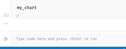
Note that if you just see three dots like this but no image:

Click the three dots, select “Change Presentation” (that was wording as of Fall 2022, it may change again…), choose “text/plain”. Then click the dots against, select “Choose Output Mimetype” again, and pick “text/html” and the figure should appear.
(Did I mention this new interface in VS Code is still a little buggy? Sorry… it is improving quickly, and it was this or teach multiple editors!)
OK, hopefully that gives you a sense of why the interactive window can be really nice, save some occasional bugs that will likely be fixed soon! Now let’s move on to Jupyter Notebooks.
Jupyter Notebooks (.ipynb files)#
Jupyter Lab can also be used to manage your Jupyter Notebooks. In order to get some experience working with a Jupyter Notebook, lets move the analysis we do in this analyze_health_and_income.py into a Jupyter Notebook.
First, open the first_jupyter_notebook.ipynb file you downloaded in VS Code.
Note: All jupyter notebooks carry the file suffix of .ipynb, regardless of what kernel they are running. This is a hangover from the old days when “jupyter” was “ipython”, so all notebooks were IPython Notebooks. But we still use the suffix .ipynb even if your notebook is running a non-Python kernel (like R, Julia, etc.). This file suffix is important because seeing that suffix is what allows VS Code to know it needs to treat the document it’s openning as a Jupyter Notebook.
Once open, follow the directions in the notebook to complete the exercise!
