Seaborn Object Recipes#
Ok, while we’re big fans of the grammer-of-graphics model of seaborn.objects, development of additional features — a version of linear regression with confidence intervals, lowess regression — has been quite slow.
To help address this, with the help of an excellent MIDS student (Ofosu Osei), we’ve created a package of extra recipes that augments seaborn.objects called seaborn_object_recipes.
To use it, just run pip install seaborn_object_recipes, then import it after seaborn:
import seaborn.objects as so
import seaborn_objects_recipes as sor
seaborn_objects_recipes Examples#
You can read about all the features of seaborn_object_recipes on the package website here, but here are a few examples of it in action.
import pandas as pd
import numpy as np
import seaborn.objects as so
import seaborn_objects_recipes as sor
import warnings

warnings.simplefilter(action="ignore", category=FutureWarning)

pd.set_option("mode.copy_on_write", True)

# Load the penguins dataset
import seaborn as sns

penguins = sns.load_dataset("penguins").dropna()
Regression with Confidence Intervals#
Here’s an example of using sor.PolyFitWithCI to plot a regression with confidence intervals.
plot = (
    so.Plot(penguins, x="bill_length_mm", y="body_mass_g")
    .add(so.Dot())
    .add(
        so.Line(), PolyFitWithCI := sor.PolyFitWithCI(order=2, gridsize=100, alpha=0.05)
    )
    .add(so.Band(), PolyFitWithCI)
    .label(
        x="Bill Length (mm)",
        y="Body Mass (g)",
        title="PolyFit Plot with Confidence Intervals",
    )
)
plot
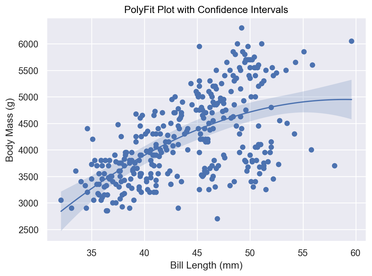
Note the need for a .add(so.Band()...) geometry. seaborn.objects thinks of the regression line as a so.Line() geometry, while the confidence interval is a so.Band() geometry.
To prevent having to fit the model twice, we use the “Walrus Operator” (:=). The Walrus Operator (turn it sideways and imagine the colon dots are eyes and the bars of the equals sign are tusks) allows the user to BOTH pass a Python object as a function argument AND save it to a variable. Here, we’re passing sor.PolyFitWithCI(order=2, gridsize=100, alpha=0.05) as the second argument in .add(so.Line(), ...) and also assigning it to the variable PolyFitWithCI, which we then use again to pass the same object in .add(so.Band(), ...). It’s a little clumsy, but works!
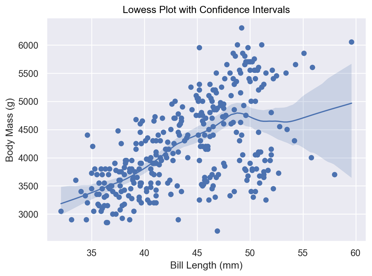
Lowess Regression with Confidence Intervals#
And here’s a lowess regression with confidence intervals!
plot = (
    so.Plot(penguins, x="bill_length_mm", y="body_mass_g")
    .add(so.Dot())
    .add(
        so.Line(),
        lowess := sor.Lowess(frac=0.4, gridsize=100, num_bootstrap=200, alpha=0.95),
    )
    .add(so.Band(), lowess)
    .label(
        x="Bill Length (mm)",
        y="Body Mass (g)",
        title="Lowess Plot with Confidence Intervals",
    )
)
plot