Plotting Zoo - with style!

Since matplotlib allows you to use style sheets to change your plots with a single line of code and those changes can entirely remake your plots. Let’s apply a style to the plots we made in our “Plotting Zoo” lesson previously to see just how dramatic that change can be with just one line of code. I’d recommend you look back at that lesson for reference before reviewing the new plots below.

%config InlineBackend.figure_format = 'retina'
import pandas as pd
import numpy as np
import matplotlib.pyplot as plt

data = pd.read_csv("data/employment-by-industry.csv")
employment = data.values[:, 1:].astype(float) / 1000
sectors = ["Healthcare", "State Gov.", "Retail", "Manufacturing", "Food & Hotel"]
years = [2018, 2019, 2020, 2021, 2022]

# APPLY THE STYLE
plt.style.use("mystyle.mplstyle")

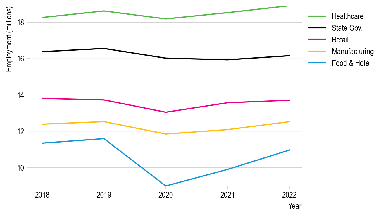
Line plot

fig, ax = plt.subplots(figsize=(6, 4))

for sector, employees in zip(sectors, employment):
    ax.plot(years, employees, label=sector)
ax.set_xlabel("Year")
ax.set_ylabel("Employment (millions)")
ax.legend(bbox_to_anchor=(1, 1), loc="upper left")
ax.set_xticks(years)

[<matplotlib.axis.XTick at 0x11f842f60>,
 <matplotlib.axis.XTick at 0x11f842f30>,
 <matplotlib.axis.XTick at 0x11f842570>,
 <matplotlib.axis.XTick at 0x11f8c1ac0>,
 <matplotlib.axis.XTick at 0x11f8c1fd0>]

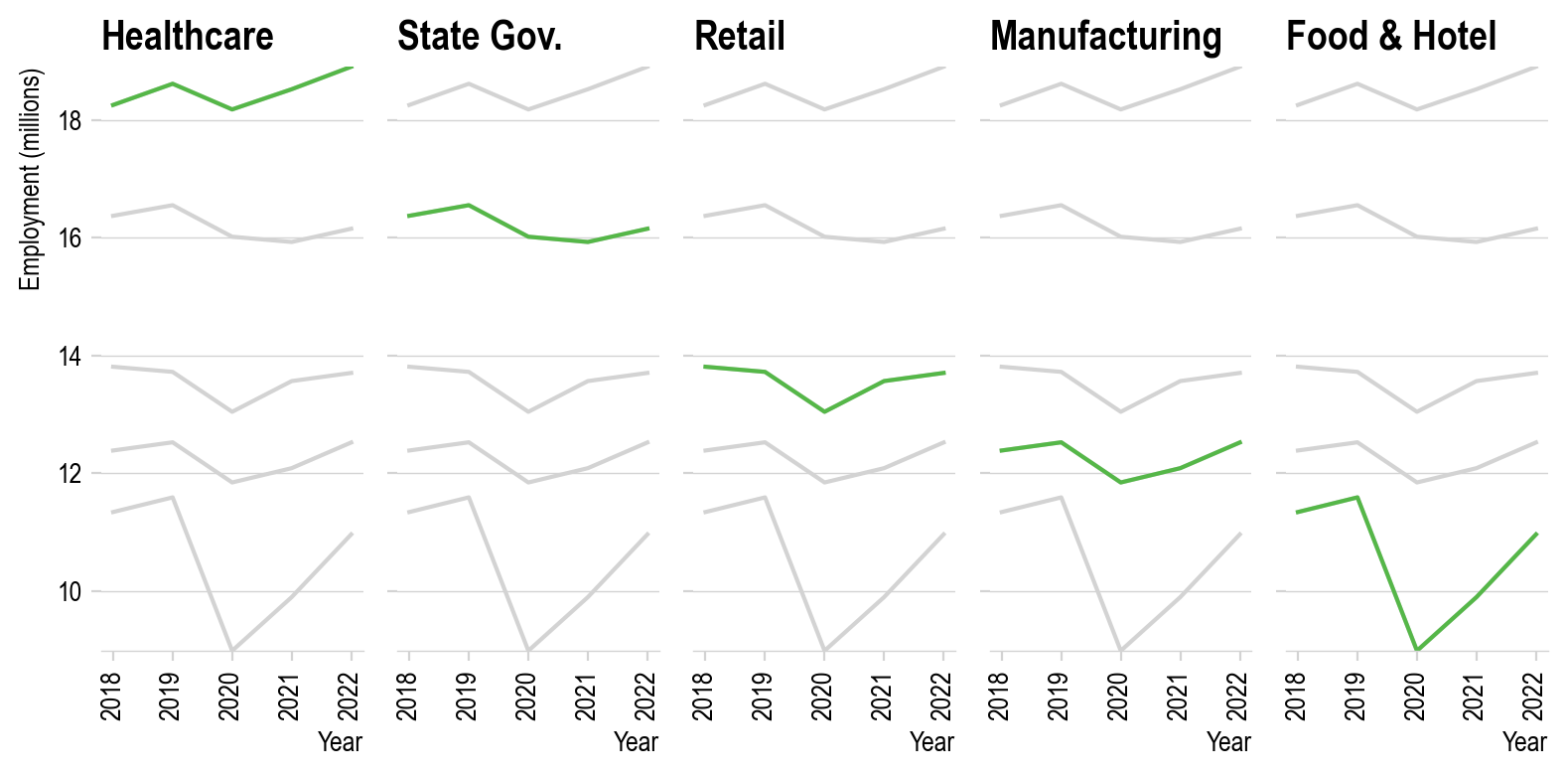
Line plot small multiples

N_sectors = len(sectors)
fig, axs = plt.subplots(
    1, N_sectors, sharey=True, figsize=(8, 4)
)  # Sharey means only the leftmost y-tick labels are shown

# Plot all the plots in grey
for ax in axs.flatten():
    for sector, employees in zip(sectors, employment):
        ax.plot(years, employees, color="lightgrey")
    ax.set_xlabel("Year")
    ax.set_xticks(years)
    ax.set_xticklabels(years, rotation=90)

# Plot one plot each in color and title the plot with that sector
for sector, employees, ax in zip(sectors, employment, axs.flatten()):
    ax.plot(years, employees)
    ax.set_title(sector)

# Only place one ylabel on the first set of Axes:
axs[0].set_ylabel("Employment (millions)")

plt.tight_layout()

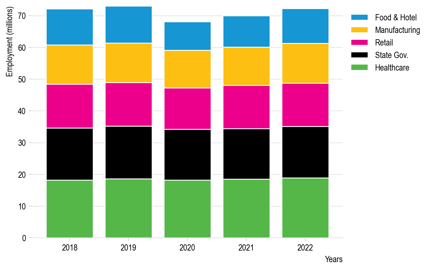
Bar plot

fig, ax = plt.subplots()

N_years = len(years)
bottom = np.zeros(
    N_years
)  # Stores the current baseline of the bars to set as the baseline for the next set of bars

for sector, employees in zip(sectors, employment):
    ax.bar(
        years, employees, label=sector, bottom=bottom, edgecolor="white"
    )  # edgecolor = 'white' places a bit of white between the bars for clarity (a personal preference)
    bottom += employees

ax.legend(
    bbox_to_anchor=(1, 1), loc="upper left", reverse=True
)  # This ensures the order matches the order in the plot from top to bottom
ax.set_xlabel("Years")
ax.set_ylabel("Employment (millions)")

Text(0, 1, 'Employment (millions)')

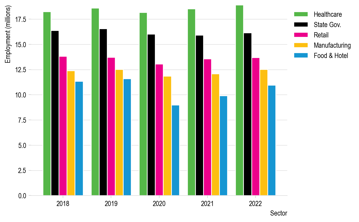
fig, ax = plt.subplots()

num_columns = len(sectors)  # Number of bars per group
num_rows = len(years)  # Number of groups

x_values = np.arange(num_rows)

bar_width = 1 / (
    num_columns + 1
)  # width of the bars. To ensure a gap between groups, this could be 1 / (N+1) where N is the number of bars per group
column_count = 0  # Count of how many sets of bars have been plotted so far

for sector, employees in zip(sectors, employment):
    offset = (
        bar_width * column_count
    )  # Offset from the x axis value for the group to the place where the bar will be centered
    ax.bar(
        x_values + offset, employees, width=bar_width, label=sector, edgecolor="white"
    )  # edgecolor = 'white' places a bit of white between the bars for clarity (a personal preference)
    column_count += 1

tick_locations = (
    x_values + (1 - offset) / 2 + bar_width
)  # Place the ticks at the center of the groups of bars
ax.set_xticks(tick_locations)
ax.set_xticklabels(years)

ax.legend(bbox_to_anchor=(1, 1), loc="upper left")
ax.set_xlabel("Sector")
ax.set_ylabel("Employment (millions)")

Text(0, 1, 'Employment (millions)')

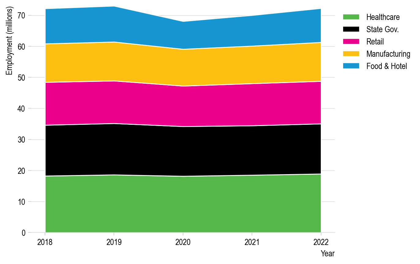
Stackplots

fig, ax = plt.subplots()

ax.stackplot(
    years, employment, labels=sectors, edgecolor="white"
)  # edgecolor = 'white' places a bit of white between the colors for clarity (a personal preference)
ax.set_xlabel("Year")
ax.set_ylabel("Employment (millions)")
ax.set_xticks(years)

ax.legend(bbox_to_anchor=(1, 1), loc="upper left")

<matplotlib.legend.Legend at 0x11fb72de0>

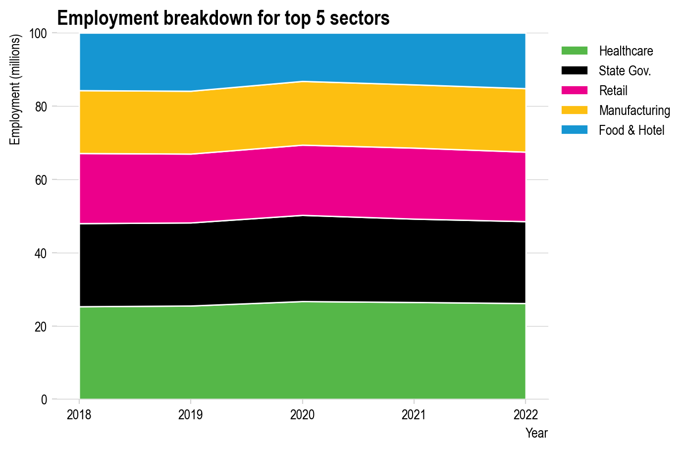
Scaled stack plots

# Convert our data to a percentage
employment_percent = employment / employment.sum(axis=0) * 100

fig, ax = plt.subplots()

ax.stackplot(years, employment_percent, labels=sectors, edgecolor="white")
ax.set_xlabel("Year")
ax.set_ylabel("Employment (millions)")
ax.set_xticks(years)
ax.set_title("Employment breakdown for top 5 sectors")

ax.legend(bbox_to_anchor=(1, 1), loc="upper left")

<matplotlib.legend.Legend at 0x11fc7f470>

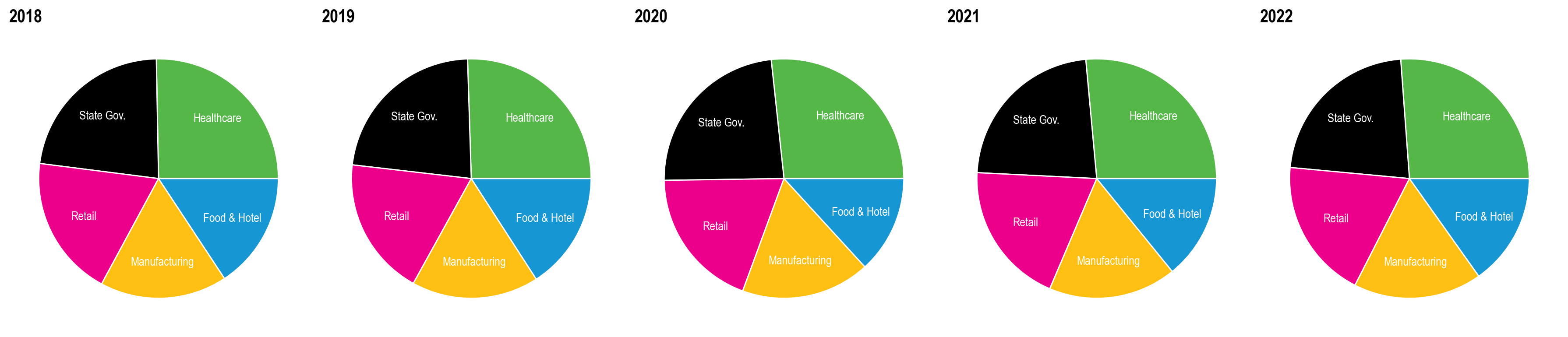
Pie charts

N_sectors = len(sectors)
fig, axs = plt.subplots(
    1, N_sectors, figsize=(18, 5)
)  # The figsize here is set sufficiently

# Plot all the plots in grey
employment_by_sector = employment.T
for year, employees, ax in zip(years, employment_by_sector, axs.flatten()):
    ax.pie(
        employees,
        labels=sectors,
        labeldistance=0.7,
        wedgeprops={"edgecolor": "white"},
        textprops={"horizontalalignment": "center", "color": "white"},
    )
    ax.set_title(year)

plt.tight_layout()

Your turn

Try change the styles yourself and see which you prefer. Try existing styles, download a new one, or create your own!