Pie charts

Pie charts are, thankfully, quite easy to make in matplotlib. Let’s revisit our example of the total grain, wheat, and barley across the three farms that we discussed in a previous lesson and plot the percentage of each that is present. Recall here that the index of the total series is the names of the types of crops.

%config InlineBackend.figure_format = 'retina'

import matplotlib.pyplot as plt

# Data to plot
crop = ["Grain", "Wheat", "Barley"]
total = [65, 193, 146]

Pie charts

Pie charts are, thankfully, quite easy to make in matplotlib. Let’s revisit our example of the total grain, wheat, and barley across the three farms and plot the percentage of each that is present. Recall here that the index of the total series is the names of the types of crops.

fig, ax = plt.subplots()

ax.pie(total, labels=crop)

([<matplotlib.patches.Wedge at 0x10ee6b260>,
  <matplotlib.patches.Wedge at 0x10ee268d0>,
  <matplotlib.patches.Wedge at 0x10ee6baa0>],
 [Text(0.962450074274041, 0.5326254354890437, 'Grain'),
  Text(-0.8889120235622774, 0.647947076825274, 'Wheat'),
  Text(0.46401849921153376, -0.9973398780703978, 'Barley')])

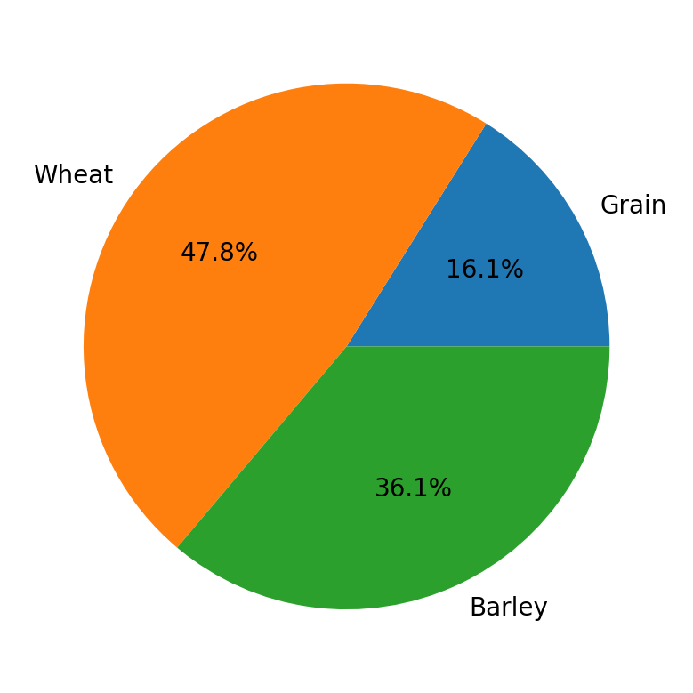
Oftentimes we want to see the percentages of each piece of the pie, and we can add that in using the autopct keyword argument, which plots text representing the percent of each of the pieces of the pie using whatever string plotting function is provided. In this case, we create a lambda function that returns the percent to 1 decimal place and has a percentage sign at the end.

fig, ax = plt.subplots()

ax.pie(total, labels=crop, autopct=lambda x: f"{x:.1f}%")

([<matplotlib.patches.Wedge at 0x10ee6bdd0>,
  <matplotlib.patches.Wedge at 0x10ee9fb60>,
  <matplotlib.patches.Wedge at 0x10ef1c410>],
 [Text(0.962450074274041, 0.5326254354890437, 'Grain'),
  Text(-0.8889120235622774, 0.647947076825274, 'Wheat'),
  Text(0.46401849921153376, -0.9973398780703978, 'Barley')],
 [Text(0.5249727677858405, 0.29052296481220563, '16.1%'),
  Text(-0.48486110376124214, 0.3534256782683312, '47.8%'),
  Text(0.2531009995699275, -0.5440035698565806, '36.1%')])

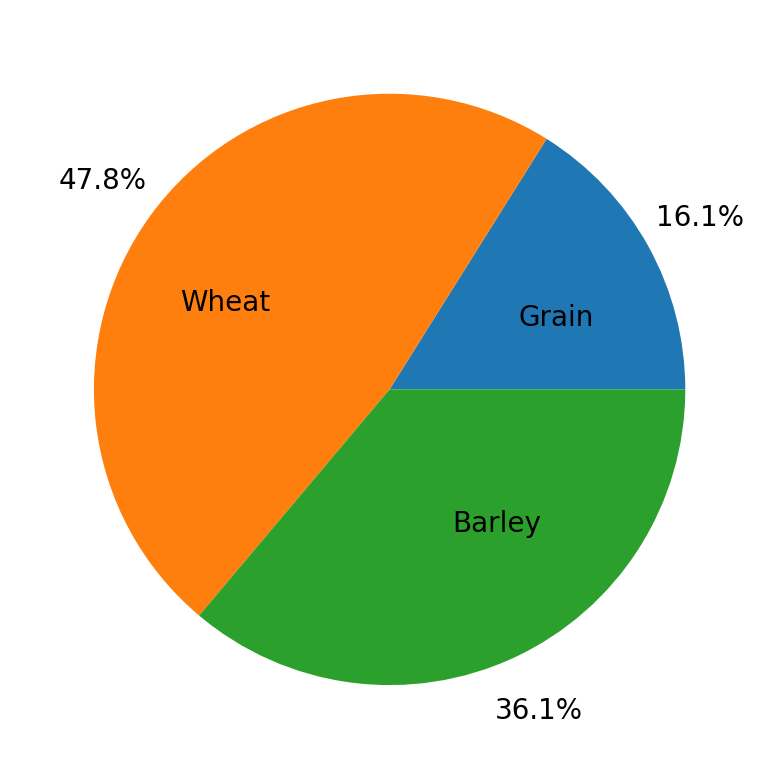
Maybe we want the name of the grain inside the plot and the percent outside the plot. We can adjust this with two keyword arguments: pctdistance, which is the relative distance along the radius of the pie where the text created by autopct is located. The edge of the pie chart is a distance of 1, so anything larger than 1 is outside the chart and anything smaller than 1 is inside the chart. There’s an analogous keyword argument for the label, labeldistance. Let’s adjust those to see how we can swap the text locations.

fig, ax = plt.subplots()

ax.pie(
    total,
    labels=crop,
    autopct=lambda x: f"{x:.1f}%",
    pctdistance=1.2,
    labeldistance=0.5,
)

([<matplotlib.patches.Wedge at 0x10ef3e810>,
  <matplotlib.patches.Wedge at 0x10ef1d3a0>,
  <matplotlib.patches.Wedge at 0x10ef3f200>],
 [Text(0.4374773064882004, 0.24210247067683802, 'Grain'),
  Text(-0.40405091980103514, 0.2945213985569427, 'Wheat'),
  Text(0.21091749964160625, -0.45333630821381715, 'Barley')],
 [Text(1.049945535571681, 0.5810459296244113, '16.1%'),
  Text(-0.9697222075224843, 0.7068513565366624, '47.8%'),
  Text(0.506201999139855, -1.0880071397131612, '36.1%')])

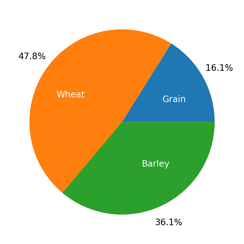
But what if we wanted to change the colors of the text? This requires a bit more knowledge of the inner workings of matplotlib, but we can see how this works by looking at the parameters that our output from the pie() method. The three returns from this method are an array of the patches that form the pie slices themselves, an array of the text objects that are the labels, and an array of the text objects that are the percentage text. To change the color of any of these we just need to iterate over them and set their color to what we’d like. Let’s set the color of all of the label names to white:

fig, ax = plt.subplots()

patches, text_label, text_percent = ax.pie(
    total,
    labels=crop,
    autopct=lambda x: f"{x:.1f}%",
    pctdistance=1.2,
    labeldistance=0.5,
)

for text in text_label:
    text.set_color("white")

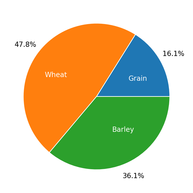
Lastly, personally, I find it visually helpful to have some space between each wedge, and this can be done by setting the edgecolor to white for the slices. This is done through the wedgeprops keyword argument which takes a dictionary of property values to apply to all of the polygons that make up the pie chart.

fig, ax = plt.subplots()

patches, text_label, text_percent = ax.pie(
    total,
    labels=crop,
    autopct=lambda x: f"{x:.1f}%",
    pctdistance=1.2,
    labeldistance=0.5,
    wedgeprops={"edgecolor": "white"},
)

for text in text_label:
    text.set_color("white")