Grouping datasets

Now that we’ve explored how to effectively combined our data into a single DataFrame, we can explore a common set of operations for summarizing data based on shared characteristics. Let’s jump in with an example. Let’s say we have the following dataset that describes the number of car sales at a dealership over three years. In that time, there were 9 employees who each worked there for a year, and different years had different numbers of employees.

import pandas as pd

pd.set_option("mode.copy_on_write", True)

sales = pd.DataFrame(
    data={
        "employee": [
            "Katrina",
            "Guanyu",
            "Jan",
            "Roman",
            "Jacqueline",
            "Paola",
            "Esperanza",
            "Alaina",
            "Egweyn",
        ],
        "sales": [14, 17, 6, 12, 8, 3, 7, 15, 5],
        "year": [2018, 2019, 2020, 2018, 2020, 2019, 2019, 2020, 2020],
    }
)
sales

	employee	sales	year
0	Katrina	14	2018
1	Guanyu	17	2019
2	Jan	6	2020
3	Roman	12	2018
4	Jacqueline	8	2020
5	Paola	3	2019
6	Esperanza	7	2019
7	Alaina	15	2020
8	Egweyn	5	2020

We want to answer two questions:

1. What year was the best for the number of sales?

2. Which year was the best for the number of sales per employee?

Let’s start with Question 1. To answer this, we need to know how many sales there were in each year. We could do this manually, summing the values of sales for each year and reporting the results; but we couldn’t do this by hand practically if this list had 1 million entries in it. This is where the groupby method shines.

Groupby:

We can use a process that is facilitated by groupby to (a) split the data into groups, (b) apply a function to the contents of each group independently, and then (c) combine the data back into a single DataFrame. The figure below shows how we can group by ‘year’, and sum the data from the ‘sales’ column, all in one simple expression.

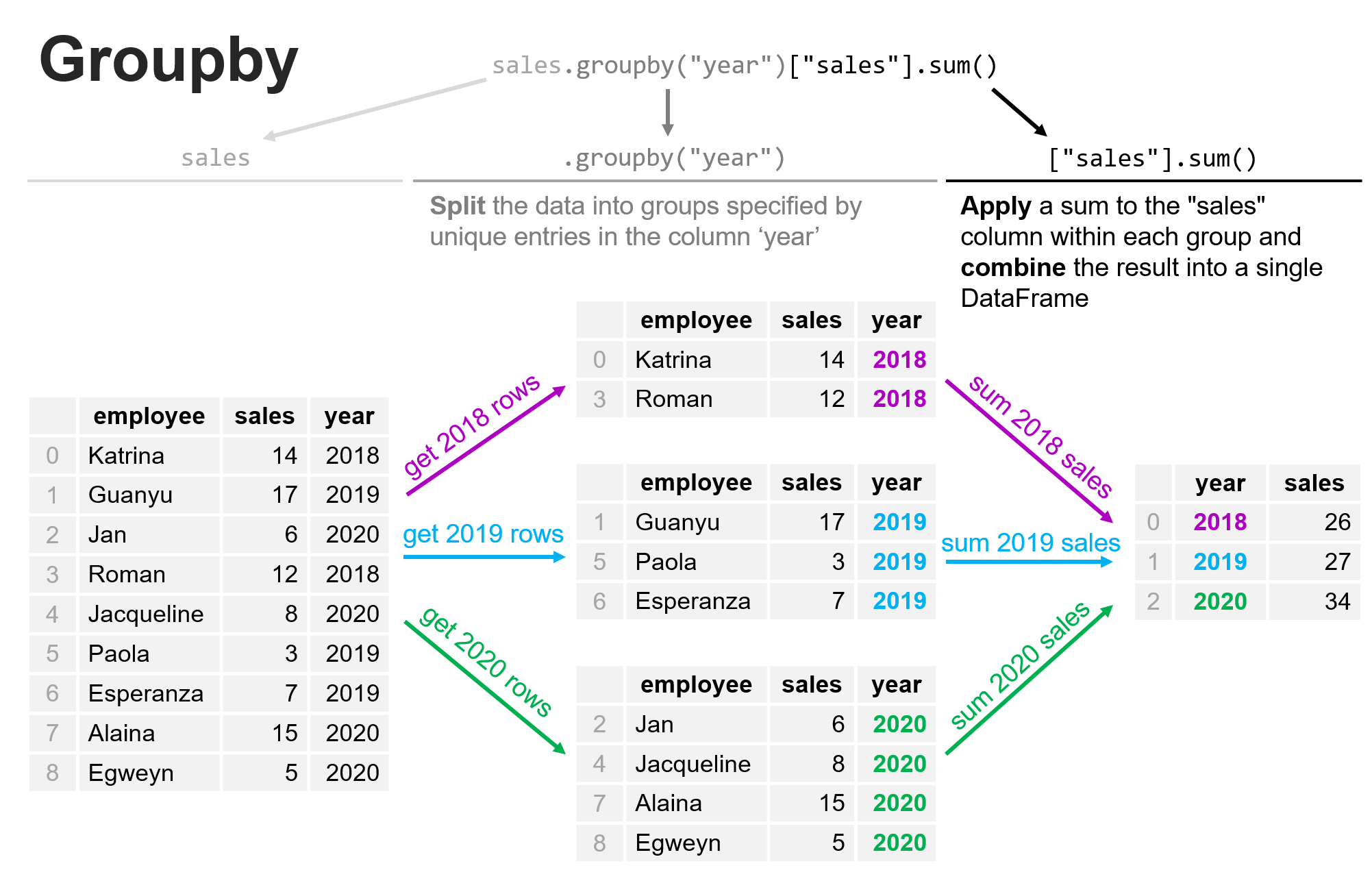
sales_by_year = sales.groupby("year")["sales"].sum()
sales_by_year

year
2018    26
2019    27
2020    34
Name: sales, dtype: int64

From the data above, we can see that 2020 was clearly the best year for sales of the 3 years considered here.

Now let’s think through Question 2, above: which year was the best for the number of sales per employee? We need some additional data here. We need the data from Question 1 on the number of sales per year, but we also need to count how many employees there were each year:

employees_by_year = sales.groupby("year")["employee"].count()
employees_by_year

year
2018    2
2019    3
2020    4
Name: employee, dtype: int64

Now let’s combine these into a single DataFram. You don’t have to do this (in fact, programmatically there are often many ways of accomplishing your objective), but it will make the data easier to probe, especially if you had a larger dataset.

question_2_data = pd.merge(sales_by_year, employees_by_year, on="year", how="left")
question_2_data

	sales	employee
year
2018	26	2
2019	27	3
2020	34	4

Now let’s compute the number of sales by employee:

question_2_data["sales_per_employee"] = (
    question_2_data["sales"] / question_2_data["employee"]
)
question_2_data

	sales	employee	sales_per_employee
year
2018	26	2	13.0
2019	27	3	9.0
2020	34	4	8.5

And there we have our answer to Question 2 - the best year for the number of sales by employee was 2018 even though the total number of sales in 2020 was higher.

Aside on as_index = False

One sometime annoying quirk of groupby is that its default behavior makes the grouped-by variable into the index of the DataFrame that’s produced such as shown below:

employees_by_year = sales.groupby("year")["employee"].count()
employees_by_year

year
2018    2
2019    3
2020    4
Name: employee, dtype: int64

employees_by_year.index

Index([2018, 2019, 2020], dtype='int64', name='year')

Here we can see that the years have become the index. You may not always want this behavior. You can always make the index back into a column using the reset_index method:

employees_by_year.reset_index()

	year	employee
0	2018	2
1	2019	3
2	2020	4

However, it’s often more convenient to simply leave it as a column in the process of applying groupby simply by setting the as_index keyword argument as shown below:

employees_by_year = sales.groupby("year", as_index=False)["employee"].count()
employees_by_year

	year	employee
0	2018	2
1	2019	3
2	2020	4

I recommend that you use as_index=False for any groupby operations unless you have a reason to do otherwise.

groupby multiple variables

Sometimes you don’t want to group by just one variable, but the unique combination of multiple variables. Consider the following example of data on the number of animals in animal shelters:

shelters = pd.DataFrame(
    data={
        "shelter_name": [
            "Helping Paws",
            "Helping Paws",
            "Helping Paws",
            "Helping Paws",
            "Feline Helpers",
            "Feline Helpers",
            "Feline Helpers",
            "Feline Helpers",
        ],
        "type": ["dog", "dog", "cat", "cat", "dog", "dog", "cat", "cat"],
        "sex": ["male", "female", "male", "female", "male", "female", "male", "female"],
        "number": [12, 31, 24, 9, 6, 2, 15, 25],
    }
)
shelters

	shelter_name	type	sex	number
0	Helping Paws	dog	male	12
1	Helping Paws	dog	female	31
2	Helping Paws	cat	male	24
3	Helping Paws	cat	female	9
4	Feline Helpers	dog	male	6
5	Feline Helpers	dog	female	2
6	Feline Helpers	cat	male	15
7	Feline Helpers	cat	female	25

In this case for each shelter, the number of dogs and cats are provided by the sex of the animal. What if we wanted to know how many dogs or cats were in each shelter? To accomplish this, if we just groupby type, it doesn’t give us what we want:

shelters.groupby(by="type", as_index=False)["number"].sum()

	type	number
0	cat	73
1	dog	51

This groups across all the shelters as well. Instead, we can group by multiple variables:

shelters.groupby(by=["shelter_name", "type"], as_index=False)["number"].sum()

	shelter_name	type	number
0	Feline Helpers	cat	40
1	Feline Helpers	dog	8
2	Helping Paws	cat	33
3	Helping Paws	dog	43

Now we can easily see how many dogs and cats each of the shelters has present.

Custom functions for combining the data (apply)

In the above examples, we used the functions sum and count as our aggregation functions for groupby by we could had used any function we’d like the operates across the grouped values. Let’s demonstrate this by showing that we could create a custom sum across our data that is 10% less than the true sum.

First let’s remind ourselves of the original data grouped by sum:

sales_by_year = sales.groupby("year", as_index=False)["sales"].sum()
sales_by_year

	year	sales
0	2018	26
1	2019	27
2	2020	34

Now let’s create our custom sum and apply it with apply:

def my_sum_10_percent_less(x):
    real_sum = sum(x)
    return 0.9 * real_sum


sales_by_year = sales.groupby("year", as_index=False)["sales"].apply(
    my_sum_10_percent_less
)
sales_by_year

	year	sales
0	2018	23.4
1	2019	24.3
2	2020	30.6

Adding grouped aggregates to the original dataset (transform)

What if we wanted to answer the question - what percent of each year’s total sales did each employee contribute? Now we could do this with our groupby result above given that we have the totals for each year, but the transform method allows us to do this seamlessly. First of all, transform allows us to transform any column in DataFrame. For example, if we wanted to double the sales numbers in the original DataFrame:

def my_transform(x):
    return sum(x)


sales_total_per_year = sales.groupby("year", as_index=False)["sales"].transform(
    my_transform
)
sales_total_per_year

0    26
1    27
2    34
3    26
4    34
5    27
6    27
7    34
8    34
Name: sales, dtype: int64

Now if we add this back into the original dataset as a column, we can see what this has done:

sales["total_by_year"] = sales_total_per_year
sales

	employee	sales	year	total_by_year
0	Katrina	14	2018	26
1	Guanyu	17	2019	27
2	Jan	6	2020	34
3	Roman	12	2018	26
4	Jacqueline	8	2020	34
5	Paola	3	2019	27
6	Esperanza	7	2019	27
7	Alaina	15	2020	34
8	Egweyn	5	2020	34

This is useful because when paired with groupby it allows us to return the grouped values in such a way that any entry with the year 2018 will have the total for 2018 as a new column. Since transform returns a Series has the same number of rows at the original DataFrame, we now have the total sales for 2018 (26) assigned to all the employees for that year (Katrina and Roman). We can now add one final column that has the percentage of sales by year for each employee:

sales["percent_by_year"] = sales["sales"] / sales["total_by_year"] * 100
sales

	employee	sales	year	total_by_year	percent_by_year
0	Katrina	14	2018	26	53.846154
1	Guanyu	17	2019	27	62.962963
2	Jan	6	2020	34	17.647059
3	Roman	12	2018	26	46.153846
4	Jacqueline	8	2020	34	23.529412
5	Paola	3	2019	27	11.111111
6	Esperanza	7	2019	27	25.925926
7	Alaina	15	2020	34	44.117647
8	Egweyn	5	2020	34	14.705882

Summary

In this lesson we explored how groupby can be used to describe and summarize data based on a shared attribute and how to customize how the data that share the attribute are aggregated. In the next lesson, we’ll extend this further to the case when we want to group according to more than one attribute.